|
Types of Accuracy
There are a number of ways in which the frequency of an oscillator can vary, all of which will affect accuracy to some degree.
Long-term accuracy relates to variations in frequency measured over a large number of cycles, anything from milliseconds to years. Any inaccuracies here will be indicated by a variation in the average output frequency.
Near-term accuracy relates to variations over just a few cycles, or even from cycle to cycle. Systems with good long-term accuracy may still show considerable variation in the near-term. Factors, which may be important include the frequency of the variation (which is often periodic in nature), the degree of variation, and the rate of change in frequency. Near-term accuracy is often referred to as "jitter" or "phase noise."
Measurement Techniques
Probably the most commonly used instrument to measure oscillator performance is a frequency counter. This instrument typically generates an aperture in time and counts the number of clock cycles occurring during that interval. Since this aperture is typically many thousands of cycles wide, it will (by definition) display an average frequency and the effects of short-term variations in frequency and/or duty cycle will be averaged out. This technique is adequate for measuring long-term variation.
A more sophisticated approach is to use a Timing Interval Analyzer (TIA, actual names may vary) which samples a large number of cycles and produces a histogram showing the distribution of a number of samples as a function of frequency. (See Figure 1.) This approach will more clearly show near-term frequency variations. This equipment is therefore useful to indicate the range and standard deviation of the output period produced by the oscillator.
The variations indicated by the TIA may be periodic or random in nature. The TIA plot does not reveal this information but an FFT will. A spectrum analyzer is a suitable instrument for this type of measurement. (See Figure 2.) Some of the more sophisticated digital oscilloscopes are capable of producing most, if not all, of the types of information described above.
Initial Accuracy (Tolerance)
This is simply the frequency at which an oscillator will run if it is operated under nominal conditions compared to its specified frequency. Typically the frequency is measured over a large number of cycles, such as with a frequency counter, so it is a measure of the oscillator's average operating frequency. For many applications this measurement is adequate for determining suitability, but as we shall see later this approach may prove inadequate for more demanding applications. Other long term stability effects (e.g., temperature or aging) will add to this initial error in a cumulative fashion.
Long-Term Stability
Temperature
Most oscillators display some sort of frequency variation with temperature. This variation may be included in a "global" tolerance specification or may be specified separately. Crystal oscillators often specify this in the form of X ppm/degree. The importance of temperature stability depends on the application. Many applications operate over a fairly narrow range of temperatures while others can accept some variation in frequency within the overall timing budget. Applications which require greater stability may necessitate higher-cost approaches such as TCXOs (temperature compensated crystal oscillators) or even crystal ovens. In some cases, frequency variation is acceptable as long as the actual deviation is known with some accuracy. Some GPS systems fall into this category. They use a temperature-sensing device to produce a correction term for the frequency variation.
Voltage
As with variations in temperature, most oscillators exhibit sensitivity to operating voltage. Again this may be included in a global tolerance specification, or may be specified separately. Obviously an oscillator with little variation over a wide voltage range is somewhat redundant for use in a system where the supply voltage is regulated within a 5% window.
Aging
This phenomenon is familiar to users of crystal-based oscillators. Over thousands of hours of normal operation, the crystal "ages," resulting in a slight change in operating frequency. The long-term effects are manifested by a change in average operating frequency and can be measured by a frequency counter. Aging is of most concern in systems, which rely on counting edges to define a real time reference. The cumulative variation is often specified as a percentage of the nominal frequency, as an absolute variation in frequency (Hz) or period (ns), or in parts per million (ppm). Crystal-based oscillators may well offer a center frequency accuracy of 150 ppm or better.
Near-Term Stability
Even if an oscillator exhibits perfect performance in terms of average output frequency, there may still be considerable variation over a smaller number of cycles, even from one cycle to the next. This short-term variation in frequency is known variously as "jitter" or "phase noise." Using a TIA, the distribution of output frequencies can be clearly seen.
Jitter components
|
There are two key components which characterize the jitter, the amplitude of the variation and, if this variation is periodic, the frequency (or frequencies) of this variation.
The amplitude of the variation corresponds to the width of the distribution shown on a TIA plot. This may be specified as the peak-to-peak range or the standard deviation (one or three sigma). Figure 1 shows such a plot for a low-cost PLL. While the center frequency is within 50 ppm of its nominal value (period of 15.15 ns), it can be seen that output periods are produced over the range of 14.9 to 15.4 ns. This corresponds to a variation of ±1.65%, which is a lot more variability than the 50 ppm specification suggests.
|
![Click here for larger image.]()
Figure 1. Example TIA trace showing center frequency and distribution of pulse widths.
|
A phase-locked loop (PLL) oscillator will typically exhibit some degree of jitter at the loop frequency resulting in a periodic variation of the output period. To see this, a spectrum analyzer plot is required.
The loop frequency is the rate at which the VCO (Voltage Controlled Oscillator) receives frequency corrections. Typically the correction signal is a sawtooth waveform which results in frequency modulation of the VCO, hence the oscillator output. Since the waveform is a sawtooth there will be components at the loop frequency and its harmonics. Figure 2 illustrates this effect. You may be surprised at all the components you see! Of course the amplitude of these components is considerably less than the fundamental but there are situations where this may produce undesirable side effects in a system.
![Figure 2. Example Spectrum Analyzer trace showing frequency components at loop frequency.]() |
Figure 2. Example Spectrum Analyzer trace showing frequency components at loop frequency. |
Why is jitter important?
Different applications have different concerns when it comes to oscillator accuracy. Somewhat surprisingly, relatively few applications really care about absolute center frequency accuracy. For example, a CPU running at 100 MHz would be most unlikely to care about a few percent of variation in frequency. Ultimately, other system timing derived from the system clock (e.g., bus timing) may impose the limit. On the other hand, "real-time" applications care primarily about average frequency. In this type of application a timing interval is measured by counting clock edges over a large number of cycles. A variation of just a few percent would make for a very inaccurate time of day clock! Since these applications are driven by average frequency, the jitter component is not important and can be ignored. Of course there are applications in telecom and broadcast television where high-center frequency is critically important but typically the performance specs will necessitate a much more sophisticated oscillator than those described here.
Other applications are more concerned with the time interval between successive clock edges, in particular the minimum interval between successive edges. In this context jitter will manifest itself as some edges appearing closer together while others appear further apart. Depending on the system timing budget this may become critical, especially if temperature effects also have to be considered. For example, when transferring data across a bus, time must be allowed for the data to be set up and stable before it can be clocked into a register. In really high-speed systems, both clock edges may be used and in this case the duty cycle of the clock also becomes important.
In other applications the variation from one cycle to the next, or across just a few cycles, is of concern. Typically this is when the clock is used for synchronization and some other circuitry is being locked to the oscillator, such as for data recovery. Too much variation from cycle to cycle and the lock may be lost.
Many telecom applications are sensitive to this type of jitter, and as a result there are many lengthy industry specifications including maximum jitter allowances as a function of jitter frequency.
In the area of data acquisition, sampling clocks such as switched capacitor or sigma-delta implementations must also be as jitter-free as possible or in-band aliasing of the sampled signal can occur, resulting in measurement errors. In this case the various frequency components of the output waveform will be of concern.,
The DS1075 EconOscillator and various other oscillator implementations are compared for jitter performance in each of these areas in the data shown later. (See "Types of Oscillators".)
Worst-Case Modeling
To ensure system integrity under all conditions all the relevant parameters mentioned above must be considered. For a real-time clock, an analysis of long term stability over the operating voltage and temperature ranges will typically be all that is required. On the other hand, over worst-case voltage and temperature scenarios a system which is clocking data on both clock edges will have to carefully consider minimum output periods and duty cycle of the clock, along with maximum access times and the associated set up and hold times of the bus.
|
What Matters Most?
By now it should be obvious that those parameters which are most important are dependent on the type of application. However, it can generally be stated that the majority of applications are very tolerant of frequency variations. Often a cumulative 5-10% accuracy will be quite sufficient.
Here are some examples of data which illustrate the effects of various types of oscillator inaccuracy.
|
![Click here for larger image.]()
Figure 3. Comparison of output periods from a DS1075 and a simple PLL.
|
The distribution of output periods is shown in Figure 3. The same PLL shown previously is compared with a DS1075. Both are running at similar frequencies, 66MHz for the PLL and 66.66MHz for the DS1075. The PLL is running at exactly the right frequency (average period = 15.15 ns), and the DS1075 is off by 10 ps (average period = 14.99 ns).
One might expect the PLL to be the more accurate device since it has a crystal reference as opposed to the DS1075 accuracy spec of only 1%, but the distribution suggests otherwise. The PLL distribution runs from 14.91 to 15.41 ns which is equivalent to +1.7%/-1.6%, the DS1075 distribution is from 14.89 ns to 15.07 ns or +0.5%/-0.7%. Even if we add the 1% frequency tolerance specified for the DS1075, this range becomes +1.5% to -1.7% which is no worse than the PLL.
So for applications where the limiting item on system performance is edge-to-edge timing, the DS1075 performs just as well as the PLL. In this type of application the ppm of the crystal is usually insignificant compared to the jitter introduced by the PLL. (Typically the system clock should be as fast as possible for maximum throughput, but the minimum period should be sufficiently high to avoid violating timing constraints.)
It is also worth noting that while both oscillators produce the same approximate minimum output period, the average frequency for the DS1075 is about 1% higher, implying a 1% greater system throughput.
The moral here is to be wary of blind acceptance of low ppm center frequency specifications!
Another feature on some test equipment allows the variation of output period to be measured over time. This is an indication of cycle-to-cycle variations and can be seen in the upper plot in Figure 4. The lower plot is the same FFT (from the 66MHz PLL) shown previously. The upper plot shows period deviations from the average over a 1µs time interval. These transitions may be of concern in applications where other circuitry has to be locked to this clock. A rapid transition could result in loss of lock, at least temporarily. In fact, excessively abrupt transitions should be avoided whenever there is any sensitivity to phase changes of the clock.
![Click here for larger image.]() |
Figure 4. Period variation and FFT for a simple PLL. |
| |
DS1075 |
555 Timer |
Crystal Oscillator* |
PLL* |
| Center Frequency Accuracy |
1% |
10% |
150 ppm |
150 ppm |
| Jitter |
<100 ps |
~10 ns |
<100 ps |
~500 ps |
| External Components |
0 |
Several |
0 |
Crystal |
| Temperature Stability |
Fair |
Poor |
Good |
Good |
| Output Enable |
Yes |
Possible |
Available |
Yes |
| Power Down |
Yes |
No |
No |
No |
| Multiple Outputs |
Yes |
No |
No |
Some |
| Frequency Range |
30kHz - 100MHz |
<500kHz |
<50MHz |
500kHz - 150MHz |
| User Reprogrammable |
Yes |
Yes |
No |
Some |
| * Typical performance. Actual performance varies according to specific device. |
Types of Oscillators
A wide variety of oscillators are available to the design engineer. These range from simple and inaccurate RC-based circuits to crystal oscillators encased in constant temperature ovens. Some of the more common implementations are outlined here, along with their key characteristics.
|
Crystal Oscillators
The ubiquitous "crystal-in-a-can" type of oscillators are found on many circuit boards. They are typified as simple to use, very accurate, and reasonably priced in the lower frequencies. Potential drawbacks include fixed operating frequencies, the need to custom order specific frequencies, and somewhat large physical size. In some applications their vulnerability to mechanical shock or vibration is of concern.
The upper trace shown in Figure 5 is from a 66.66MHz crystal oscillator. To achieve this frequency the crystal is probably being operated in a harmonic mode. Points to note include the center frequency, which is exact (15 ns), and the narrow distribution (80 ps), showing none of the spreading indicative of a PLL-based approach.
|
![Click here for larger image.]()
Figure 5. Histograms for a crystal oscillator and the DS1075.
|
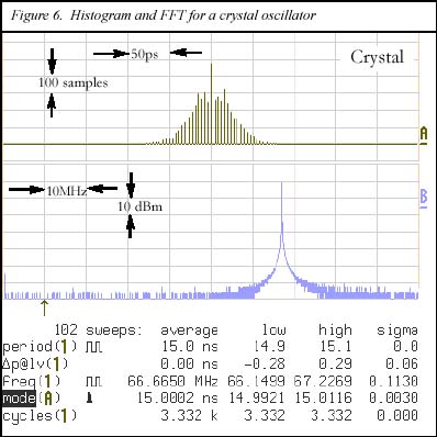
Figure 6. Histogram and FFT for a crystal oscillator.
|
For comparison, the lower trace shows the DS1075, which also features a narrow distribution (120 ps), but the center frequency is slightly off (10 ps). An expanded view of the histogram and an FFT plot are shown in Figure 6. Not surprisingly, the FFT is very clean.
From a purely timing-based point of view the crystal is ideal, offering accurate center frequency and low jitter. Drawbacks to this approach are in areas such as size, additional features and programmability. Furthermore, crystals operating at frequencies above approximately 30MHz (the highest commonly available fundamental crystal frequency) become increasingly expensive.
|
|
Crystal-Based Phase-Locked Loops (PLLs)
These devices combine the frequency stability of a crystal (at least for long term stability) with the ability to synthesize a number of different output frequencies from a single fixed-crystal frequency. This is achieved by dividing the crystal frequency down to arrive at a loop frequency, which is in turn compared to the divided-down output of a voltage controlled oscillator (VCO). Any frequency difference is detected by a phase detector, the output of which is filtered and used to provide a control voltage for the VCO. Therefore the output frequency can be altered to any integer multiple of the loop frequency by simply changing the value of the divider between the output and the phase comparator. Although the phase comparator output is filtered, some component of the error signal manifests itself as frequency modulation of the output. The result is that, although the center frequency of the oscillator may be very accurate, jitter components of several percent may exist on the output.
|
Figure 7. Frequency histogram and FFT plot for another PLL.
|
The characteristics of one type of PLL have been shown in Figures 1 and 2. Figure 7 illustrates the characteristics of another type of PLL. This one is configured to multiply the input frequency (an 11.059MHz crystal) by a factor of six, resulting in a 66.35MHz output. It will be noticed that the histogram is bi-modal but the average frequency is still accurate at 15.07 ns. Again, some spreading is evident with output periods ranging by over 220 ps, or about 1.5% variation.
![Click here for larger image.]()
Figure 8. Peak-to-peak jitter for two different PLLs.
|
The FFT is also cleaner than the previous PLL, but still shows components all the way down to the megahertz range.
Figure 8 shows the peak-to-peak jitter for both PLLs; the upper trace is for the device shown previously (Figures 1 and 2) and the lower trace for the second PLL (Figure 7). It will be noticed that there is a significant difference in peak-to-peak jitter for the two devices.
|
It should be noted that there are many types of PLL available today, some of which offer much better jitter performance than those shown here. However, these two PLLs were selected as being representative of the low cost PLLs likely to be considered for this type of application. Higher-performance PLLs also carry higher price tags.
|
RC Oscillators
These are very simple oscillators requiring just a resistor and capacitor to set the frequency. Either a ubiquitous 555 timer circuit or a Schmitt-trigger inverter can be used to build a simple oscillator. Of course, while the RC time constant may vary considerably with temperature and voltage, with this error adding to the initial component tolerance, this is probably the cheapest way to build an oscillator. 555-based timers are limited to operating frequencies below 1MHz (manufacturer's recommendation) but the Schmitt trigger-type can be used at higher frequencies. This type of implementation should be used only when the crudest of oscillators are needed.
|
![Click here for larger image.]()
Figure 9. Histogram for DS1075 and 555 at 500kHz.
|
|
DS1075 EconOscillator Family
This family of oscillators from Dallas Semiconductor needs no external timing components and offers accuracies of better than 1% over temperature and voltage. Since they are not PLL-based, there are few jitter components in the output. This can be clearly seen in Figure 10 which shows the histogram, FFT and period-to-period variation. The relatively narrow distribution, lack of spurious output frequency components and modest variation from cycle to cycle indicate a very (near-term) stable oscillator.
|
![Click here for larger image.]()
Figure 10. Histogram, FFT and peak-to-peak jitter plots for the DS1075.
|
Furthermore, they are available in small footprint packages including 150-mil SOICs and (in the future) µSOPs. These devices are modestly priced and also offer the option of user-reprogrammability for a number of discrete frequencies up to 100MHz. Sufficiently accurate for most applications, this family offers low cost, low component count and flexibility within possibly the smallest footprint in the industry.
For more information, application notes, data sheets and product selection guides for the DS1075 and entire Dallas Semiconductor oscillator family, please visit our web site at http://www.dalsemi.com/products/stc/index.html
DS1075 Demo and Programming Kit
Evaluating or programming engineering prototypes is easy with the DS1075K Demo and Programming Kit[1075k.pdf - MISSING]. Included in the kit is the PC Board, samples of the DS1075 in DIP packages (2 of each master frequency) and Windows-based software. The board also supports the 3-pin DS1065 EconOscillator/Divider and the 3-volt DS1073 EconOscillator/Divider[1073.pdf - MISSING]. Space is provided on the board for SOIC and/or TO-92 sockets, or a simple adapter can be made to use the existing DIP socket.
The kit makes it easy to program the devices for preparing engineering prototypes or just to evaluate device capabilities. Control of the various operating modes is possible via software or onboard switches, and BNC sockets allow the outputs to be monitored or an external input to be provided. (Note: The board is optimized for programming purposes and is less than optimum for generating clean output waveforms at higher frequencies.)
![Click here for larger image.]() |
![Click here for larger image.]() |
Evaluation, programming and prototyping on the DS1075K Kit is easy right out of the box. It's done via the graphic user interface of the Windows-compatible software or using the switches on the PC board. |
![Click here for larger image.]()
Figure 11. Fixtures, made for each chip and crystal, were tested on the LeCroy model LC534AM.
|
Other Types of Oscillators
All the oscillators mentioned above are modestly priced and perfectly acceptable for many types of applications. There are applications where a higher degrees of accuracy is essential. These applications are served by several types of crystal-based oscillators (VCXOs, TCXOs, etc.) and some high-performance PLLs. These applications are beyond the scope of this document.
There are also applications where an actual oscillator is not required. A number of microcontrollers offer on-chip oscillators which simply need an external reference such as a crystal or ceramic resonator. Assuming no additional features are required, this low-cost approach works well for many applications.
|
Other Considerations
The ultimate performance achieved with all the above approaches can be affected by layout and decoupling considerations. Any time high frequencies are involved, switching noise and supply or ground bounce can produce additional errors. Good decoupling techniques (high frequency capacitors mounted as close as possible to device pins) should always be employed.
We developed special fixtures for each device tested to try and obtain as clean an output as possible. (See Figure 11.) Care was taken to terminate the outputs correctly, and good decoupling was provided as close to the device as possible. All lead lengths were as short as possible and there was plenty of ground plane provided.
Output loading and termination is also important. Unwanted reflections on cables to the test equipment can cause erroneous results. In real-world applications, care must be taken in board layout to ensure no mismatches are present.
Temperature affects different types of oscillators in different ways. To a first approximation, the crystal-based types are immune to variations in temperature (except for the very low ppm types), one of the attractions in using a crystal reference. RC oscillators, on the other hand, are very susceptible to temperature variations as the component values will vary. The DS1075 fits between these extremes, however on-chip compensation keeps the variation to less than 1%. As always, the specific data sheets should be consulted for any particular type of oscillator.
For the above reasons, none of the various devices measured (except the DS1075) have been specified by name. In addition, we were only able to measure a small sample, which may or may not have been representative of production devices. We recommend reading the manufacturer's specifications very carefully and conducting your own measurements when necessary to determine which type of oscillator is best-suited for a given application.
Test Equipment
All the data shown in this report was taken with a LeCroy digital oscilloscope, model LC534AM. It features 1GHz bandwidth and up to 2G samples per second. Similar results could be obtained from various other types of equipment, but a very high sampling rate is essential for cycle-to-cycle measurements.
|