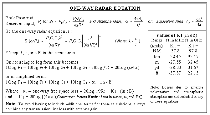
The one-way (transmitter to receiver) radar equation is derived in this section. This equation is most commonly used in RWR or ESM type of applications. The following is a summary of the important equations explored in this section:
Recall from the Power Density Section that the power density at a distant point from a radar with an antenna gain of Gt is the power density from an isotropic antenna multiplied by the radar antenna gain.
Power density from radar, 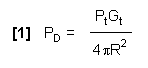
If you could cover the entire spherical segment with your receiving antenna you would theoretically capture all of the transmitted energy. You can't do this because no antenna is large enough. (A two degree segment would be about a mile and three-quarters across at fifty miles from the transmitter.)
A receiving antenna captures a portion of this power determined by it's effective capture Area (Ae). The received power available at the antenna terminals is the power density times the effective capture area (Ae) of the receiving antenna.
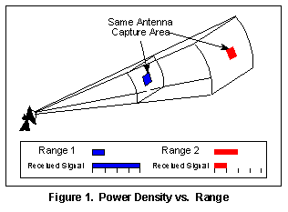 For a given receiver
antenna size the capture area is constant no matter how far it
is from the transmitter, as illustrated in Figure 1.
For a given receiver
antenna size the capture area is constant no matter how far it
is from the transmitter, as illustrated in Figure 1.
This concept is shown in the following equation:
Peak Power at Receiver input,
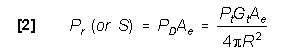
which is known as the one-way (beacon) equation
In order to maximize energy transfer between an antenna and
transmitter or receiver, the antenna size should correlate with
frequency. For reasonable antenna efficiency, the size of an antenna
will be greater than ![]() /4. Control of beamwidth shape
may become a problem when the size of the active element exceeds
several wavelengths.
/4. Control of beamwidth shape
may become a problem when the size of the active element exceeds
several wavelengths.
The relation between an antenna's effective capture area (Ae) or effective aperture and it's Gain (G) is:
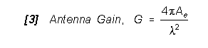
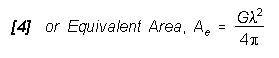
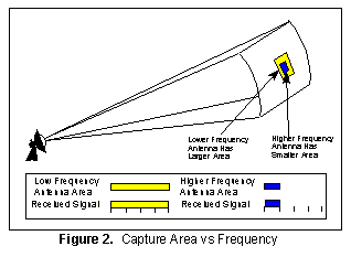 Since the effective
aperture is in units of length squared, from equation [3], it
is seen that gain is proportional to the effective aperture normalized
by the wavelength. This physically means that to maintain the
same gain when doubling the frequency, the area is reduced by
1/4. This concept is illustrated in Figure 2.
Since the effective
aperture is in units of length squared, from equation [3], it
is seen that gain is proportional to the effective aperture normalized
by the wavelength. This physically means that to maintain the
same gain when doubling the frequency, the area is reduced by
1/4. This concept is illustrated in Figure 2.
If
equation [4] is substituted into equation [2], the following relationship
results:
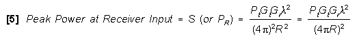
This is the signal calculated one-way from a transmitter to a receiver. For instance, a radar application might be to determine the signal received by a RWR, ESM, or an ELINT receiver. It is a general purpose equation and could applied to almost any line-of-sight transmitter to receiver situation if the RF is higher than 100 MHZ.
The free space travel of radio waves can, of course, be blocked, reflected, or distorted by objects in their path such as buildings, flocks of birds, chaff, and the earth itself.
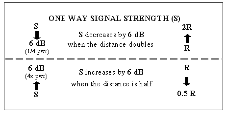 As illustrated in Figure
1, as the distance is doubled the received signal power decreases
by 1/4 (6 dB). This is due to the R2 term in equation
[5].
As illustrated in Figure
1, as the distance is doubled the received signal power decreases
by 1/4 (6 dB). This is due to the R2 term in equation
[5].
To illustrate this, blow up a round balloon and draw a square on the side of it. If you release air so that the diameter or radius is decreased by 1/2, the square shrinks to 1/4 the size. If you further blow up the balloon, so the diameter or radius is doubled, the square has quadrupled in area.
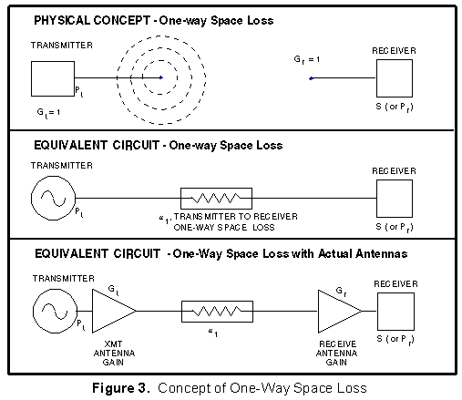
One-way space loss (![]() ) is illustrated as a physical
concept and as an equivalent circuit in Figure 3.
) is illustrated as a physical
concept and as an equivalent circuit in Figure 3.
The one-way free space loss factor (![]() ), (sometimes
called the path loss factor) is given by the term (4
), (sometimes
called the path loss factor) is given by the term (4![]() R2)(4
R2)(4![]() /
/![]() 2)
or (4
2)
or (4![]() R /
R /![]() )2. As shown in
Figure 3, the loss is due to the ratio of two factors:
)2. As shown in
Figure 3, the loss is due to the ratio of two factors:
(1)
the effective radiated area of the transmit antenna, which
is the surface area of a sphere (4![]() R2)
at that distance (R), and
R2)
at that distance (R), and
(2) the effective
capture area (Ae) of the receive antenna which has
a gain of one.
If a receiving antenna could capture
the whole surface area of the sphere, there would be no spreading
loss, but a practical antenna will capture only a small part of
the spherical radiation. Space loss is calculated using isotropic
antennas for both transmit and receive, so ![]() is
independent of the actual antenna.
is
independent of the actual antenna.
Using Gr = 1 in equation [11] in the Antenna
Introduction Section, Ae = ![]() 2/4
2/4![]() .
Since this term is in the denominator of
.
Since this term is in the denominator of ![]() , the
higher the frequency (lower
, the
higher the frequency (lower ![]() ) the more the space loss.
Since Gt and Gr are part of the one-way
radar equation, S (or Pr) is adjusted according to
actual antennas as shown in the last portion of Figure 3. The
value of the received signal (S) is:
) the more the space loss.
Since Gt and Gr are part of the one-way
radar equation, S (or Pr) is adjusted according to
actual antennas as shown in the last portion of Figure 3. The
value of the received signal (S) is:
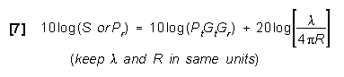
To convert this equation to dB form, it is rewritten as:
Since ![]() = c / f, equation [7] can be rewritten
as:
= c / f, equation [7] can be rewritten
as:
Where the one-way free space loss,![]() , is defined as:
, is defined as:
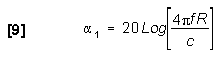
The signal received equation in dB form is:
The one-way free space loss,![]() , can be given
in terms of a variable and constant term as follows:
, can be given
in terms of a variable and constant term as follows:
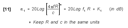
| Values of K1 (dB) | ||
|
Range (units) |
f 1 in MHz K 1 = |
f 1 in GHz K 1 = |
| NM | 37.8 | 97.8 |
| km | 32.45 | 92.45 |
| m | -27.55 | 32.45 |
| yd | -28.33 | 31.67 |
| ft | -37.87 | 22.13 |
Note: To avoid having to include additional terms for these
calculations, always combine any transmission line loss with antenna
gain.
|
A VALUE FOR THE ONE-WAY FREE SPACE LOSS ( |
|
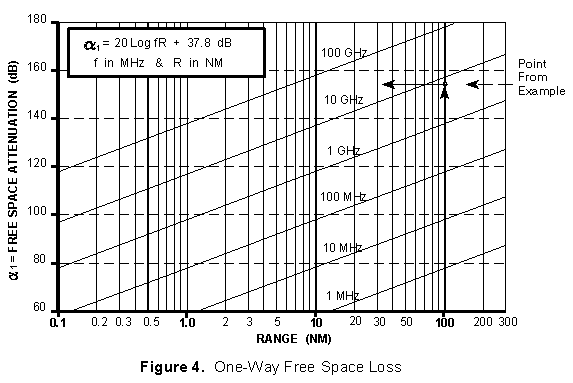
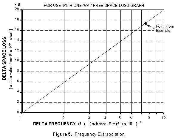
(a) The One-way Free Space Loss graph (Figure 4). Added accuracy can be obtained using the Frequency Extrapolation graph (Figure 5) |
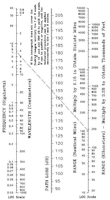
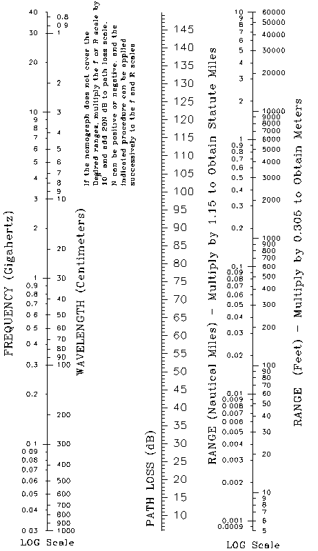
| (b) The space loss nomograph (Figure 6 or 7) |
|
(c) The formula for |
|
(One-Way Space Loss Nomograph for distances greater than 10 nautical miles) |
|
(One-Way Space Loss Nomograph for distances less than 10 nautical miles) |
FOR EXAMPLE:
Find the value of the one-way free space loss,![]() , for
an RF of 7.5 GHz at 100 NM.
, for
an RF of 7.5 GHz at 100 NM.
(a) From Figure 4, find 100 NM on the X-axis and estimate where
7.5 GHz is located between the 1 and 10 GHz lines (note dot).
Read ![]() as 155 dB. An alternate way would be to read the
as 155 dB. An alternate way would be to read the
![]() at 1 GHz (138 dB) and add the frequency extrapolation
value (17.5 dB for 7.5:1, dot on Figure 5) to obtain the same
155 dB value.
at 1 GHz (138 dB) and add the frequency extrapolation
value (17.5 dB for 7.5:1, dot on Figure 5) to obtain the same
155 dB value.
(b) From the nomogram (Figure 6), the value of ![]() can
be read as 155 dB (Note the dashed line).
can
be read as 155 dB (Note the dashed line).
(c) From the equation 11, the precise value of ![]() is
155.3 dB.
is
155.3 dB.
Remember,![]() is a free space value. If there is atmospheric
attenuation because of absorption of RF due to certain molecules
in the atmosphere or weather conditions etc., the atmospheric
attenuation is in addition to the space loss (refer to the RF
Atmospheric Absorption Section).
is a free space value. If there is atmospheric
attenuation because of absorption of RF due to certain molecules
in the atmosphere or weather conditions etc., the atmospheric
attenuation is in addition to the space loss (refer to the RF
Atmospheric Absorption Section).

Figure 8 is the visualization of the losses occurring in one-way radar equation. Note: To avoid having to include additional terms, always combine any transmission line loss with antenna gain. Losses due to antenna polarization and atmospheric absorption also need to be included.
RWR/ESM RANGE EQUATION (One-Way)
The one-way radar (signal strength) equation [5] is rearranged to calculate the maximum range Rmax of RWR/ESM receivers. It occurs when the received radar signal just equals Smin as follows:
In log form:
[13]![]() 20log Rmax = 10log Pt + 10log
Gt - 10log Smin - 20log f + 20log(c/4
20log Rmax = 10log Pt + 10log
Gt - 10log Smin - 20log f + 20log(c/4![]() )
)
and since K1 = 20log{4![]() /c times conversion
units if not in m/sec, m, and Hz}.
/c times conversion
units if not in m/sec, m, and Hz}.
[14]![]() 10log Rmax = 1/2[ 10log Pt
+ 10log Gt - 10log Smin - 20log f -
K1]
10log Rmax = 1/2[ 10log Pt
+ 10log Gt - 10log Smin - 20log f -
K1] ![]() ( keep Pt and Smin in same
units)
( keep Pt and Smin in same
units)
If you want to convert back from dB, then Rmax is approximately 10MdB/20, where MdB is the resulting number in the brackets of equation 14.
From Receiver Sensitivity / Noise Section , Smin is related to the noise factor S:
[15]![]() Smin = (S/N)min (NF)KToB
Smin = (S/N)min (NF)KToB
The one-way RWR/ESM range equation becomes:

RWR/ESM RANGE INCREASE AS A RESULT OF A SENSITIVITY INCREASE
As shown in equation [12] 1/Smin is proportional to Rmax2 Therefore, -10 log Smin is proportional to 20 logRmax and the table below results:
% Range Increase: Range + (% Range Increase) x Range
= New Range
i.e., for a 6 dB sensitivity increase,
500 miles +100% x 500 miles = 1,000 miles
Range Multiplier: Range x Range Multiplier = New Range i.e., for a 6 dB sensitivity increase 500 miles x 2 = 1,000 miles
|
dB Sensitivity Increase |
% Range Increase |
Range Multiplier |
dB Sensitivity Increase |
% Range Increase |
Range Multiplier |
|
+ 0.5 1.0 1.5 2 3 4 5 6 7 8 9 |
6 12 19 26 41 58 78 100 124 151 182 |
1.06 1.12 1.19 1.26 1.41 1.58 1.78 2.0 2.24 2.51 2.82 |
10 11 12 13 14 15 16 17 18 19 20 |
216 255 298 347 401 462 531 608 694 791 900 |
3.16 3.55 3.98 4.47 5.01 5.62 6.31 7.08 7.94 8.91 10.0 |
RWR/ESM RANGE DECREASE AS A RESULT OF A SENSITIVITY DECREASE
As shown in equation [12] 1/Smin is proportional to Rmax2 Therefore, -10 log Smin is proportional to 20 logRmax and the table below results:
% Range Decrease: Range - (% Range decrease) x Range
= New Range
i.e., for a 6 dB sensitivity decrease,
500 miles - 50% x 500 miles = 250 miles
Range Multiplier: Range x Range Multiplier = New Range i.e., for a 6 dB sensitivity decrease 500 miles x .5 = 250 miles
|
dB Sensitivity Decrease |
% Range Decrease |
Range Multiplier |
dB Sensitivity Decrease |
% Range Decrease |
Range Multiplier |
|
- 0.5 - 1.0 - 1.5 - 2 - 3 - 4 - 5 - 6 - 7 - 8 - 9 |
6 11 16 21 29 37 44 50 56 60 65 |
0.94 0.89 0.84 0.79 0.71 0.63 0.56 0.50 0.44 0.4 0.35 |
-10 - 11 - 12 - 13 - 14 - 15 - 16 - 17 - 18 - 19 - 20 |
68 72 75 78 80 82 84 86 87 89 90 |
0.32 0.28 0.25 0.22 0.20 0.18 0.16 0.14 0.13 0.11 0.10 |
Example of One-Way Signal Strength:
A 5 (or 7) GHz radar has a 70 dBm signal fed through a 5 dB loss
transmission line to an antenna that has 45 dB gain. An aircraft
that is flying 31 km from the radar has an aft EW antenna with
-1 dB gain and a 5 dB line loss to the EW receiver (assume all
antenna polarizations are the same).
Note: The respective transmission line losses will be combined
with antenna gains, i.e.
-5 + 45 = 40 dB, -5 - 1 = -6 dB, -10 + 5 = -5 dB.
(1) What is the power level at the input of the EW receiver?
Answer (1): Pr at the input to the EW receiver
= Transmitter power - xmt cable loss + xmt antenna gain - space
loss + rcvr antenna gain - rcvr cable loss.
Space loss (from figures 4 through 7) @ 5 GHz =
20 log f R + K1 = 20 log (5x31) + 92.44 = 136.25
dB.
Therefore, Pr = 70 + 40 - 136.25 - 6 = -32.25 dBm
@ 5 GHz
(Pr = -35.17 dBm @ 7 GHz since ![]() = 139.17
dB)
= 139.17
dB)
(2) If the received signal is fed to a jammer with a
gain of 60 dB, feeding a 10 dB loss transmission line which is
connected to an antenna with 5 dB gain, what is the power level
from the jammer at the input to the receiver of the 5 (or 7) GHz
radar?
Answer (2): Pr at the
input to the radar receiver = Power at the input to the EW receiver+
Jammer gain - jammer cable loss + jammer antenna gain - space
loss + radar rcvr antenna gain - radar rcvr cable loss .
Therefore, Pr = -32.25 + 60 - 5 - 136.25 + 40 =
-73.5 dBm @ 5 GHz.
(Pr = -79.34 dBm @ 7 GHz since ![]() = 139.17
dB and Pt = -35.17 dBm).
= 139.17
dB and Pt = -35.17 dBm).
This problem continues in sections on the Two-Way Radar Equation, Constant Power (Saturated) Jamming, and Constant Gain (Linear) Jamming.